By courtesy of Juan Carlos Aguilar’s Numerical Calculus course at ITAM.

Context and summary of this blog post

This is the first project that I did using LaTeX! The power iteration algorithm is one of the algorithms that I enjoyed most during my undergraduate studies. I believe that it is elegant and simple. In this post we will describe the algorithm with an adequate context and an argument showing what it does and why it works. At the end we include some code in Python so that you can get even more familiarized with the algorithm.

Definitions and context.

Dominant eigenvalue of a matrix: Let \(A\in \mathbb{R}^{n\times n}\) be a diagonalizable matrix over \(\mathbb{C}\), and \(\lambda_{1},\lambda_{2},\dots,\lambda_{n}\in \mathbb{C}\) be its corresponding eigenvalues. \(\lambda_{j}\) is the dominant eigenvalue of A if and only if

Remark:

we will assume that we have a matrix \(A\),which is diagonalizable. Hence, without loss of generality, let´s suppose that \(\lambda_{1}\) is a dominant eigenvalue for our diagonalizable matrix A.

We say that \(\lambda_{1}\) is the only dominant eigenvalue of A if and only if \(|\lambda_{1}|>|\lambda_{j}| \text{ for all } j=2,\dots,n.\)

Approximation to the (only) dominant eigenvalue of a real squared matrix (if it exists)

In this section we´ll discuss the power iteration algorithm focusing in \(\mathbb{R}\), however, the ideas can be extended to \(\mathbb{C}\).

Let \(A\in \mathbb{R}^{n\times n}\) be a diagonalizable matrix over \(\mathbb{R}\) and \(\lambda_{1},\lambda_{2},...,\lambda_{n}\in\mathbb{R}\) be the corresponding eigenvalues.

Suppose that \(\lambda_{1}\) is the only dominant eigenvalue of A. Furthermore, without loss of generality we can write: \(|\lambda_{1}|>|\lambda_{2}|\geq|\lambda_{3}|\geq\dots\geq|\lambda_{n}|.\)

Since \(A\) is diagonalizable in \(\mathbb{R}\), there exist linearly independent eigenvectors of \(A\), \(\vec{v_{1}}, \vec{v_{2}},\dots,\vec{v_{n}} \in \mathbb{R}^{n}\), corresponding to the eigenvalues

\(\lambda_{1},\lambda_{2},...,\lambda_{n}\), respectively and form a basis of \(\mathbb{R}^{n}\).

Let \(\vec{u_{0}}\in\mathbb{R}^{n}-\{\vec{0}\}\) be an arbitrary vector.

Since \(\{\vec{v_{1}},\dots,\vec{v_{n}}\}\) is a basis of \(\mathbb{R}^{n}\), there exist constants \(\alpha_{1},\alpha_{1},\dots,\alpha_{n} \in \mathbb{R}\) such that:

Multiplying both sides by \(A\):

And since \(\vec{v_{i}}\) is an eigenvector of \(A\) corresponding to the eigenvalue \(\lambda_{i}\), then by definition of eigenvector we get:

Again, multiplying by \(A\) in both sides, using the same argument as above we get: \(\begin{equation} A^2\vec{u_{0}}= \sum_{i = 1}^n\alpha_{i}\lambda_{i}^2\vec{v_{i}}. \end{equation}\)

Proceeding by induction, we get:

for all \(k \in\mathbb{N}\).

Dividing both sides by \(\lambda_{1}^k\) (remember that \(\lambda_{1}\) is the only dominant eigenvalue of A by hypothesis):

And since \(0\leq|\lambda_{n}|\leq|\lambda_{n-1}|\leq\dots\leq|\lambda_{2}|<|\lambda_{1}|\), then dividing all the inequalities by \(|\lambda_{1}|>0\), we get that \(0\leq\left|\frac{\lambda_{n}}{\lambda_{1}}\right|\leq\left|\frac{\lambda_{n-1}}{\lambda_{1}}\right|\leq\dots\leq\left|\frac{\lambda_{2}}{\lambda_{1}}\right|<1,\)

if and only if \(0\leq\bigl\vert\frac{\lambda_{n}}{\lambda_{1}}\bigl\vert^k\leq\bigl\vert\frac{\lambda_{n-1}}{\lambda_{1}}\bigl\vert^k\leq\dots\leq\bigl\vert\frac{\lambda_{2}}{\lambda_{1}}\bigl\vert^k<1 \text{ for all } k\in\mathbb{N}.\)

Therefore

Going back to the equation that we obtain by induction, and taking limits in both sides we have that:

Using the fact that \(\lambda_1\) is a dominant eigenvalue, in the limit, this equation simplifies to:

This suggests that for a big \(k \in \mathbb{N}\) we obtain the following approximation: \(\begin{equation} \frac{1}{\lambda_{1}^k}A^k\vec{u_{0}}\approx\alpha_{1}\vec{v_{1}}. \end{equation}\)

Here it is worth to pause and make a couple of observations:

1. We picked \(\vec{u_{0}}\) to be an arbitrary vector in \(\mathbb{R}^{n}\). However, \(\vec{u_{0}}\) needs to satisfy that \(\alpha_{1}\) is different form 0 so that the last approximation is different from \(\vec{0}\), since \(\vec{0}\) is not an eigenvector by definition.

2. The hole point of all the argument above is to motivate an algorithm that approximates the only dominant eigenvalue of A (i.e.\(\lambda_{1}\)), which we don´t know a priori and actually want to approximate, assuming that it exists.

3. A useful property of eigenvectors worth to recall: Let \(A\in\mathbb{R}^{n\times n}\) and suppose that \(\vec{v_{1}}\in\mathbb{R}^{n}\) is an eigenvector of \(A\), then \(\alpha\vec{v_{1}}\) is also an eigenvector of A for all \(\alpha\in \mathbb{R}-\{0\}\). Moreover, from the proof of this statement it follows that \(\vec{v_{1}}\) and \(\alpha\vec{v_{1}}\) have the same associated eigenvalue of \(A\). Considering the last remark, \(\frac{A^k\vec{u_{0}}}{||A^k\vec{u_{0}||}}\) is parallel to \(\frac{1}{\lambda_{1}^k}A^k\vec{u_{0}}\) (given that we are just scaling the vector \(A^k\vec{u_{0}}\)) and thus \(\frac{A^k\vec{u_{0}}}{||A^k\vec{u_{0}||}}\) tends to an eigenvector of A associated to the dominant eigenvalue \(\lambda_{1}\) as \(k\xrightarrow{}\infty\).

Power iteration algorithm: a pseudocode

Inputs: \(A\), \(\vec{u_{0}}\), \(maxNumIter\), \(Tol\).

Output: \(\ell_{k}\), \(\vec{u}_{k}\).

1.- \(k \leftarrow 1\)

2.- \(\textbf{While } k<maxNumIter:\)

3.- \(\vec{u_{k}} \leftarrow\) \(\frac{A\vec{u}_{k-1}}{\big\|A\vec{u}_{k-1}\big\|}\)

4.- \(\ell_{k}\leftarrow \vec{u}_{k}^T A\vec{u}_{k}\)

5.- \(\textbf{If } \frac{\big\|A\vec{u}_{k}-\ell_{k}\vec{u}_{k}\big\|}{\big\|A\vec{u_{k}}\big\|}\leq Tol: \textbf{ Break while}\)

6.- \(\textbf{Else:}\)

7.- \(k\leftarrow k+1\)

8.- \(\textbf{End if}\)

9.- \(\textbf{End while}\)

10.- \(\textbf{Return } \ell_{k},\vec{u}_{k}.\)

Where \(\big\| \big\|\) denotes the Euclidean norm function for vectors in \(\mathbb{R}^n\). Notice that the initial \(\vec{u_{0}}\) must satisfy \(A\vec{u_{0}}\neq\vec{0}\).

Why does the algorithm work?

We will show that

We need some auxiliary lemmas to achive that goal. We will use the notation \(\big\| \big\|\) generically to refer to the Eucledian norm. Recall that in the case of real numbers in one dimension, it is simply the absolute value. Firstly, consider the following proposition.

Proposition

Let \(\{\vec{a}_k\}_{k=1}^{\infty}\) and \(\{\vec{b}_k\}_{k=1}^{\infty}\) be two sequences of vectors in \(\mathbb{R}^{n}\) such that

for some \(\vec{a}, \vec{b}\in \mathbb{R}^{n}\).Then

Proof

We begin by applying the triangle inequality.

Next we apply the Cauchy-Schwarz inequality:

Now, since \(\{\vec{a}_k\}_{k=1}^{\infty}\) converges, then it is bounded. On the other hand, by our hypotheses,

With this we can conclude (using the Squeeze theorem) that

This is equivalent to our desired result:

As a corollary of this proposition we can show that \(\begin{equation}\lim_{k\to\infty}\ell_k=\lambda_1.\end{equation}\)

We next describe how to note this.

If \(\vec{w}\) is an eigenvector of \(A\) with norm equal to \(1\), such that \(A\vec{w}=\lambda_1\vec{w}\), then

which is an expression similar to the one that we saw in our auxiliary proposition. It should definitely be familiar.

By the argument that we gave before the pseudocode,

This is becasue \(\vec{w}\text{ and }-\vec{w}\) are both eigenvectors of \(A\) of norm \(1\) such that their corresponding eigenvalue is \(\lambda_1\). Without loss of generality we assume that

Indeed, if it were the case that

we can simply take \(\vec{q}:=-\vec{w}\) and present all the ideas in terms of \(\vec{q}\).

It should also be clear from the pseudocode that the power iteration algorithm generates a sequence \(\{\vec{u}_k\}_{k\in \mathbb{N}}\) of unitary vectors, that is, \(\|\vec{u}_k\|=1\text{ for all }k \in \mathbb{N}.\)

So notice that once we have that

then

Therefore, by our auxiliary proposition, we have that

And we are finished! Thank you for making it this far! I hope you enjoyed the argument, which involves many interesting ideas from linear algebra.

Code in Python

We present an implementation of some iterations of the algorithm. Only for practical purposes and to get a better hands-on understanding. Perhaps not the most efficient implementation. But it should be helpful to improve the understanding of the algorithm.

import numpy as np
from matplotlib import pyplot as plt #necessary libraries
def plotConvergence(N,C, u_0):
    #N is the number of iterations that we wish to make
    #u_0 the initial vector
    #C is the matrix
    iterations=list(range(1,N+1))
    print(iterations)
    convergence=[]
    for i in range(N):
        u_0=np.dot(C,u_0)/np.linalg.norm(np.dot(C,u_0))
        l=np.dot(np.dot(u_0.transpose(),C),u_0)
        #print(l)#if we want to debug or see the generated sequence
        convergence.append(l[0])
    # Plotting
    plt.rcParams.update({'font.size': 12})
    plt.figure(figsize=(10, 6))
    plt.plot(iterations, convergence, label=r'Trajectory of $\ell_k$', linewidth=2.5)
    plt.axhline(y = max(abs(np.linalg.eig(C)[0])), color = 'r', linestyle = '--', label=r'$\lambda_1$') # this works properly assuming that the dominant eigenvalue is positive
    plt.xlabel('Iteration', fontsize='large')  # Using LaTeX notation for xlabel
    plt.ylabel(r'Value of $\ell_k$', fontsize='large')  # Using LaTeX notation for ylabel
    plt.legend(title='Convergence to the dominant eigenvalue', fontsize='large', title_fontsize='large')
    plt.xlim(1, N)
    plt.ylim(0, 10)
    plt.xticks(fontsize='large', ticks=[i for i in range(N+1)])
    plt.yticks(fontsize='large', ticks=[i for i in range(0,10)])# may need to adjust this for better visualization depending on the case
    plt.grid(False)
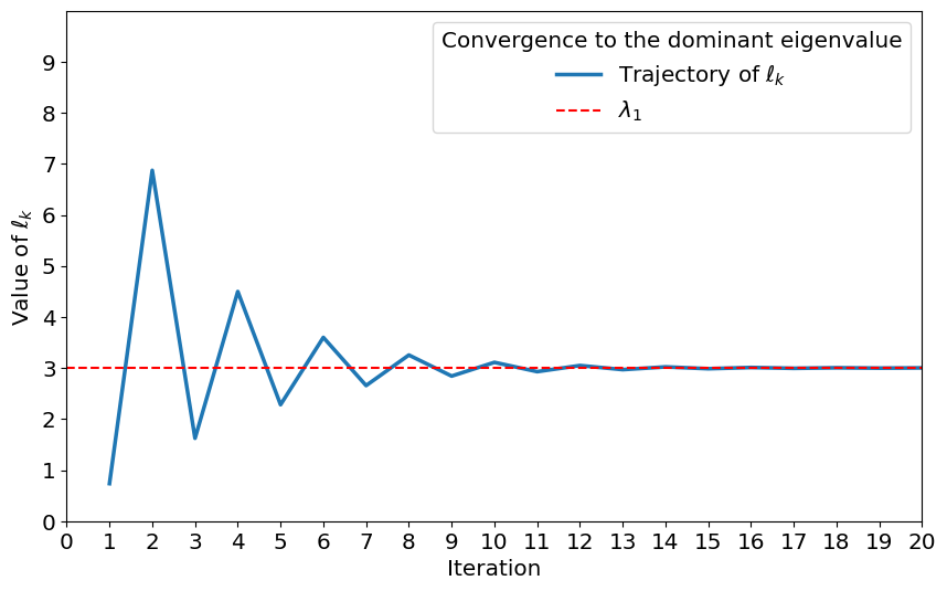
    plt.show()

As an example to try the plot function consider

#defining a matrix
B=np.array([[-1,-19,-4],[0,-2,0],[0,15,3]])
print(B)
print(B.shape)
print(np.linalg.eig(B))
#eigenvalues of B are -1,3, and 2. So our algorithm should approximate to 3.
plotConvergence(20,B, np.array([[1],[1],[1]]))

You should obtain the following plot:

Iterations of the power iteration algorithm generating a sequence that converges to the dominant eigenvalue.