This is joint work with Julieta Rivero and Rodrigo Villela.
In this blog post we will summarize our project where we used linear regression models to make predictions with real-world data.
Context
The NYC subway system (which is administrated by the Metropolitan Transportation Authority, also known as the MTA) publishes data from the usage of the services that it provides, which can be accessed here or here. We used this data to determine how the subway traffic patterns changed throughout the city due to the global pandemic. We built regression models which predict the usage decline per neighborhood. Indeed, as you might expect, the pandemic caused a huge decline in the subway rides across all New York City. The government of the City of New York has a data culture which allows us to undertand the city beyond conventional ways. We take advantage of this situation to get a deeper understanding of the relationship between the metro traffic and the demographic characteristics of the neighborhoods in NYC.
Data analysis
Our data is divided by neighborhoods in NYC. We have access to the daily rides in each of the metro stations in the city. We compared the average number of daily rides in each station between 2019 and 2020, and grouped each station to the neighborhood that they belong. We obtained a decline percentage by comparing the average daily metro rides in each neighborhood in 2019 and 2020. This is the response variable, which we refer to as \(\textbf{var_res}\).
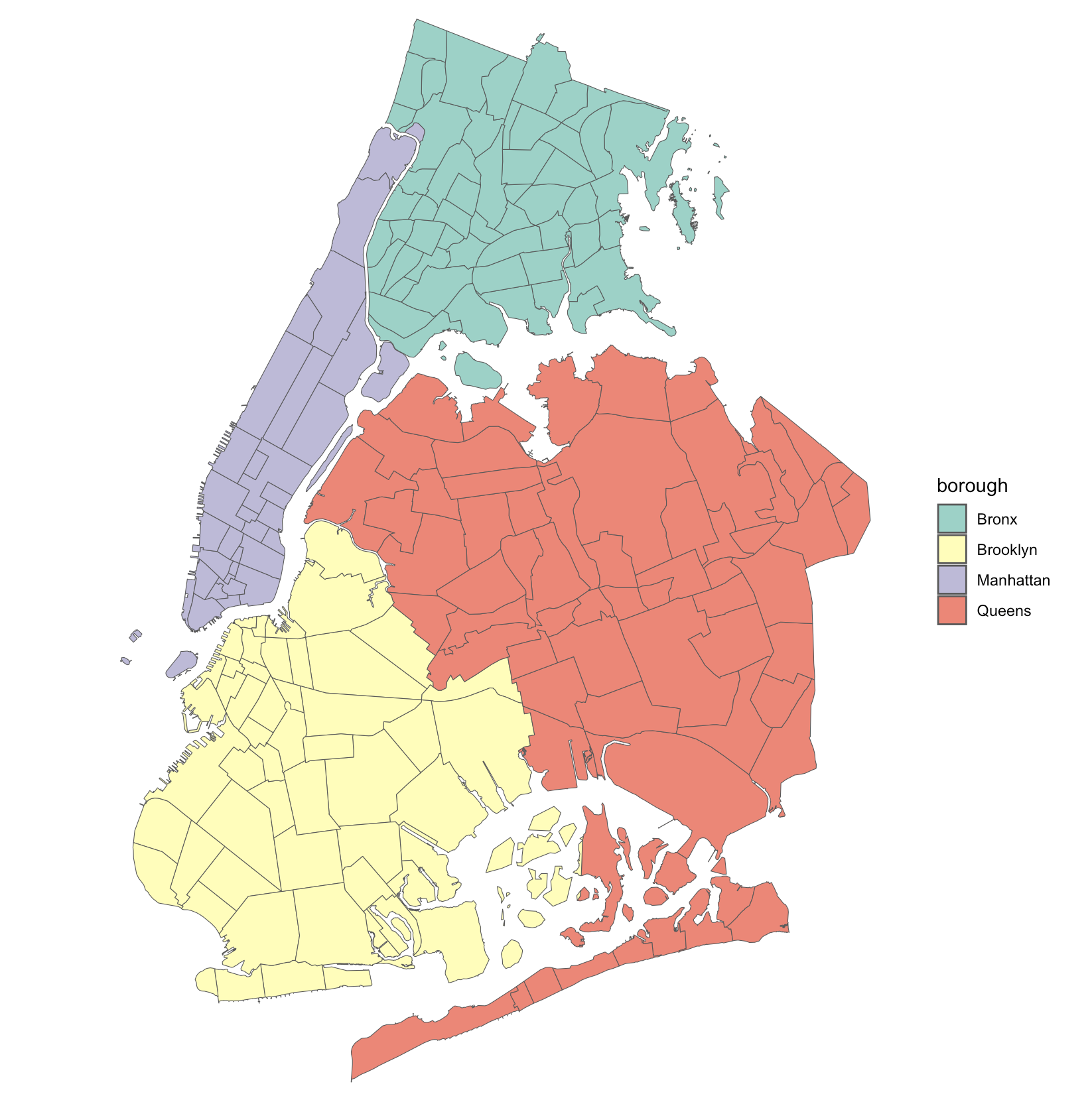 Map of NYC divided by neighborhoods in the city’s boroughs excluding Staten Island.
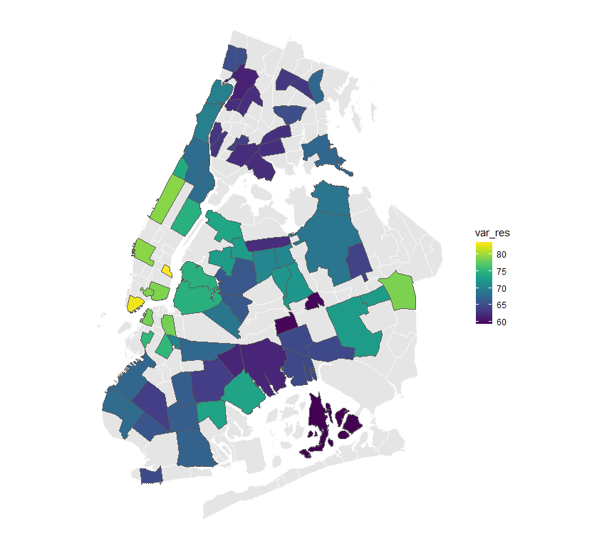 Heat map of the change in the use of the subway system after the pandemic.
We can appreciate that the neighborhood that experienced the greatest decline in the average metro usage was the Financial District of NYC, which is located at the southern tip of Manhattan. Comparing 2019 and 2020, the average daily metro usage was reduced in more than 80%.
Heat map of the change in the use of the subway system after the pandemic.
We can appreciate that the neighborhood that experienced the greatest decline in the average metro usage was the Financial District of NYC, which is located at the southern tip of Manhattan. Comparing 2019 and 2020, the average daily metro usage was reduced in more than 80%.
We considered many explanatory variables and we did a deep data analysis. Here we only present a brief picture of such analysis to summarize the project.
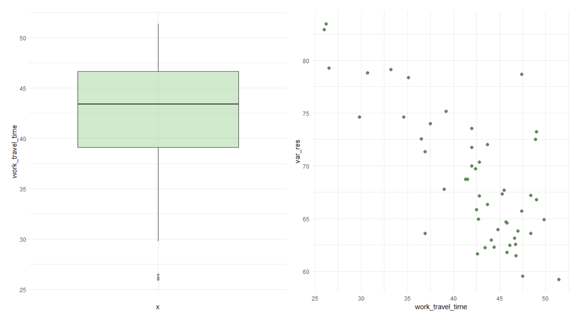 Average time to work (in minutes) for people in each neighborhood in relation to the response variable.
We can clearly appreciate a negative linear relationship between the variables. A possible reason for this relationship might be that for people whose time to work is very close, they can easily substitute the metro for walking or bycicle, for example, given that their commute to work is likely very short.
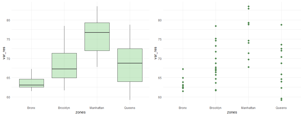 Change in the use of the subway divided by zones in NYC.
We can see that on average, the subway use got reduced the most in Manhattan. Queens has a lot of variance in the response variable, due to the fact that the whiskers in its box plot are very large. Whereas we see that the Bronx had low changes in the use of the subway with low variance.
Variables
We take distict and neighborhood as synonyms throughout the desctiption of the feature variables (predictive variables). These are some of the variables that we had in the data.
-
\(\textbf{born_nys}:\) percentage of the population on the neighborhood who were born in NYC. By definitition, this variable takes values in \([0,100]\).
-
\(\textbf{prc_car_free}\): percentage of living places in the neighborhood that do not have a car. Takes values in \([0,100]\).
-
\(\textbf{disabled_pop}\): percentage of the population in the distirct who have certain disability.
-
\(\textbf{foreign_pop}\): percentage of people in the neighborhood who are foregin.
-
\(\textbf{homeownership_rate}\): percentage of living places such that the owner of the place lives in it.
-
\(\textbf{houses_children}\): porcentage of houses in which there is at least one person younger than 18 years old.
-
\(\textbf{housing_units}\): number of housing units in the neighborhood.
-
\(\textbf{work_travel_time}\): average time (in minutes) to work for a person living in the neighborhood.
-
\(\textbf{income}\): average anual income for a peron in the district (reported in terms of 2020 us dollars).
-
\(\textbf{population}\): number of people living in the district.
-
\(\textbf{pop_65}\): percentage of habitants in the district who are older than 65 years old.
-
\(\textbf{pop_density}\): Population density. We constructed this variable by computing the number of habitants in the district per square mile and dividing it by 1,000.
-
\(\textbf{poverty_rate}\):percentage of people in the neighborhood who live in poberty.
-
\(\textbf{public_housing_prc}\): percentage of living places which are subsidized by the NY government.
-
\(\textbf{houses_park}\): percentage of living units in the neighborhood that have a park 14 miles or closer.
-
\(\textbf{crime_rate}\): number of crimes which resulted in jail for every \(1,000\) people 16 years old or older. As an example, the biggest value that we have in the dataset is 23.5. Multiplying it by 100,000 and dividing it by 1000 we obtain the number of people who went to jail for every 100,000 people. In this exaple we get that \(2,350\) people of 16 years old or older went to jail for every \(100,000\) persons in that age range. That is, \(2.35\%\) of the habitants older than 15 years old went to jail for some crime during 2020.
-
\(\textbf{unemployent_rate}\): unemployment rate in the neighborhood.
-
\(\textbf{income_cat}\): this a categorical version of the variable \(\textbf{income}\). It is divided into 4 categories according to income thresholds that we fixed. It is divided into: low, medium, medium-high, and high income. To choose the thresholds we used the quantiles of the income variable: the first quantile US \(\$49,460\) , the median of \(\$57,680\) usd and the third quantile of \(\$71,920\)usd.
-
\(\textbf{zones}\): Categorical variable dividing the neighborhoods according to their location: Bronx, Brooklyn, Manhattan and Queens.
Prediction strategy
We randomly selected 15% of the neighborhoods and kept them to test the model. We trained the model with the 85% of the remaining neighborhoods.
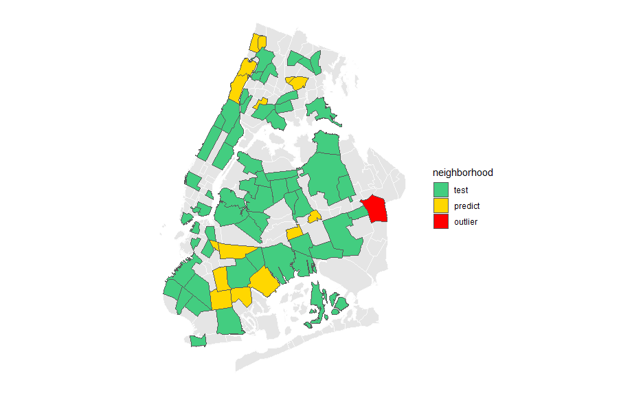 Green neighborhoods were used only for training. Yellow neighborhoods were not used for training and were used to test the performance of the model. We identified that Queens Village’s change in the use of the subway was an outlier observation.
Regression model
We implemented a classic regression model of the following form:
\[Y_i=\beta_0+\beta_{1}X_{1,i}+\dots\beta_{p-1}X_{p-1,i}+\epsilon_{i}\quad,\]where we suppose that
\[\begin{equation}\epsilon_{i}\sim N(0,\sigma^2),\quad \forall i\in \{1,\dots n\}\end{equation}\] \[\begin{equation}Cov(\epsilon_{i},\epsilon_{j})=0 \quad \forall i,j\in \{1,\dots n\} , i\neq j\end{equation}\] \[\begin{equation}\mathbf{\beta}:=\begin{bmatrix} \beta_{0} \\ \beta_{1} \\ \vdots \\ \beta_{p-1} \end{bmatrix},\end{equation}\]\(\mathbf{\beta}\) is the vector of unknown coefficients; additionally we assume that the explanatory variables are not constant for each \(i\). On the other hand, the least squares estimator of \(\mathbf{\beta}\) for the multiple regression model has the form
\[\begin{equation}\mathbf{\hat{\beta}}=(X'X)^{-1}X'\textbf{Y},\end{equation}\]where \(X\) is the design matrix and \(\textbf{Y}\) is the vector containing the response variables.
Notice that the existence of such estimator requires the matrix \(X'X\) to be invertible. In order to guarantee the invertibility of \(X'X\) we need the matrix \(X\) to have a full rank, that is, all the columns in \(X\) should be linearly independent. Whenever two explanatory variables are strongly correlated or any predictive variable has low variance, this can induce numerical problems when trying to determine the inverse matrix \(X'X\). This is why we consider the exploratory data analysis to be an imporatnt part of our project. It is also important to validate the assumptions of the model, for example, the constant variance in the errors assumption, also known as homoscedasticity. This is something that we also considered when building our linear models.