
This is joint work with my colleagues Diego Velazquez and Marcelino Sanchez.
This project is a natural extension to the project where we predicted the metro activity in NYC, because in such project we did not account for spatial correlation, whereas in this project our model allows us to account for the spatial correlation of the data.
Context
The government of the City of Boston runs a very modern approach focused on a data culture to monitor and improve the quality of life in the city and it has available open data website which offers data gathered by the Boston’s Police Department about crimes happening in the city. Anlayze Boston also reports census data for Boston’s districts, containg detailed information about Boston’s depographic characteristics. Among other things, this site offers information about the kind of crime, location and time in which the crime happened.
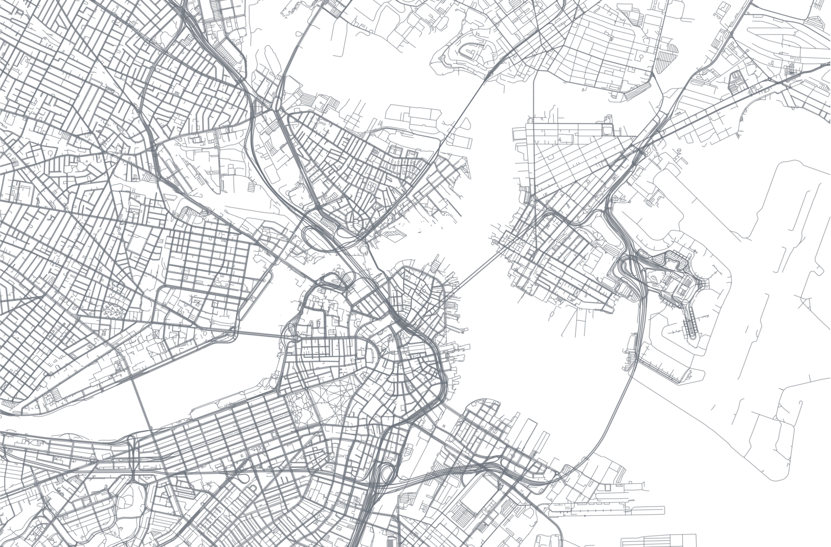 A map of Boston’s streets.
We created spatial regression models with a bayesian approach to determine the predictive capacity of demographic variables to determine crime rates for each of Boston’s districts.
Variables
We used the dataset of the crimes that occured during 2022 in the City of Boston reported by the Boston Police Department. This dataset not only includes crimes but many other kind of activities that are reported to the police such as suicides, use of drugs, etc. We restricted the data to observations that were interpretable forms of crime such as murder, shooting, larceny, shoplifting, valdalism, etc. We only used the observations that we considered that would help us get an insight about the crime situation in Boston. We constructed the response variable following the procedure that we present next.
We had two datasets: the crimes in 2022 and demographic charactersitics of the 22 districts in Boston collected in the census. Both datasets are availale in Analyze Boston. The crimes datset contains the location of the crime (in coordinates), district in which the crime occured, type of crime, time at which it was reported to the police, among others. We assigned a centroid to each of the city’s district, by selecting a point that we considered to be central within the district. We then assigned a label to each crime determined by the closest centroid. Finally, we counted how many crimes we had per district and divided them by the population size acccording to the census. This was done so that our crime rates account for the population size in each district.
In notation, if i ∈ {1, . . . , 22} is the i-th district in Boston and there occured
\(Z_i\) ∈ \(\mathbb{N}\) crimes in 2022 and according to the census of 2019, there were
\(M_i\) ∈ \(\mathbb{N}\) people in the i-th district, then we took \(Y_i := \frac{Z_i}{M_i}\) ∈ (0, ∞).
\(Y_i\) tells us the crime rate in district \(i\): the number of crimes per capita in 2022 realtive to 2019’s population.
Actually, given the nature of the data, and as we would expect to have more people than crimes in each neighborhood, then
\(Y_i\) ∈ (0, 1) ∀i ∈ {1, . . . , 22}. In order to adjust the model and work in all \(\mathbb{R}\), we consider an invertible transformation
where \(s_i\) ∈ \(\mathbb{R}^2\) are the coordinates of the i-th district (the centroid).
Hence, we consider our response variable as crime rates in a logarithmic scale.
With respect to the feature variables, the 2019 census of Boston offers a lot of details about each district. For example, distance to the closest park for each home within each district, average annual income in usd, average time to work, proportion of houses that own a car, etc.
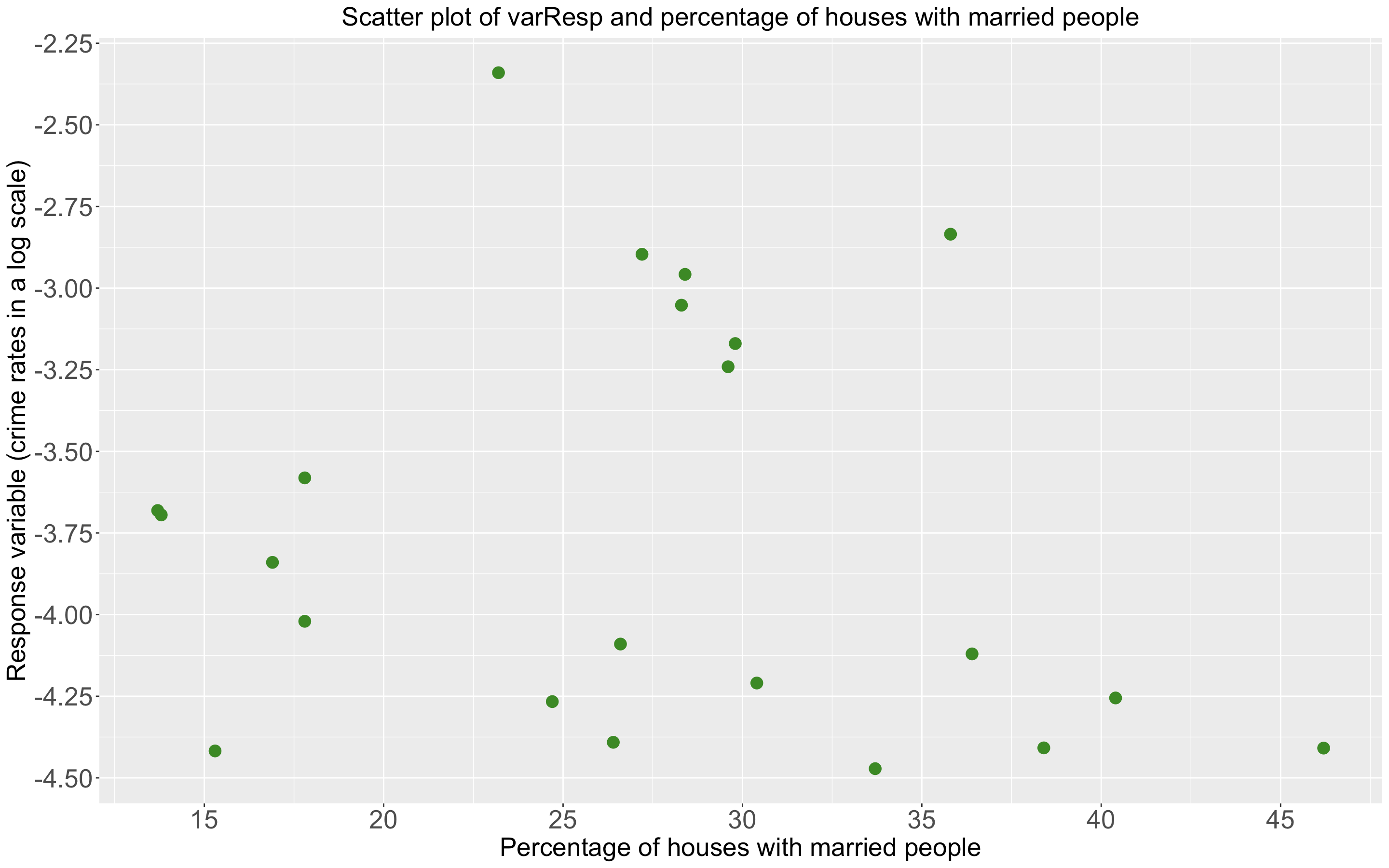 Scatter plot showing the response variable and the percentage of houses with a married couple in each district.
These two variables have a correlation of -0.15969. Though not quite strong, it is interesting to note that the correlation is negative.
Scatter plot showing the response variable and the percentage of houses with a married couple in each district.
These two variables have a correlation of -0.15969. Though not quite strong, it is interesting to note that the correlation is negative.
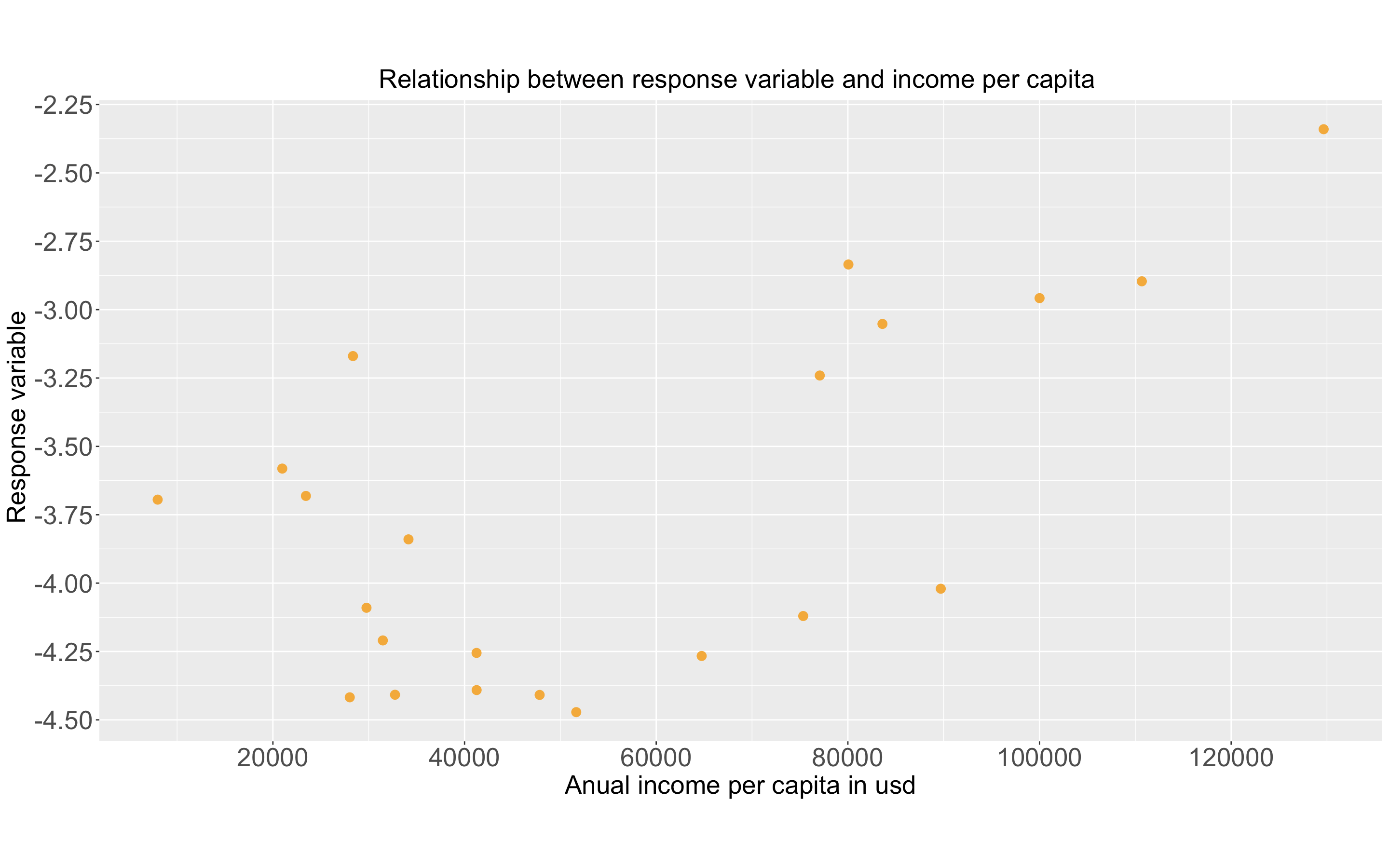 Scatter plot showing the response variable and income per capita in each neighborhood in Boston.
These two variables are strongly correlated, they actually have a correlation of 0.61378.
We could explore further this approach, or even a correlation matrix, which we included in the original work as part of the exploratory data analysis. But this is only a brief summary of the work to keep it documented in an ordered and aesthetic manner.
Here’s a list of some of the variables that we considered for the second model that we used:
percentageUndergrads: percentage of people in the district that have an undergraduate degree.
PercentageMasters: porcentage of people in the district that hold a masters degree.
PercentageMarried: percentage of properties (houses/apartments) in the district such that a married couple lives in it.
incomePerCapita: average annual income per person in the neighborhood.
metroTren: percentage of people in the neighborhood whose main transport is the metro or the train.
Data analysis
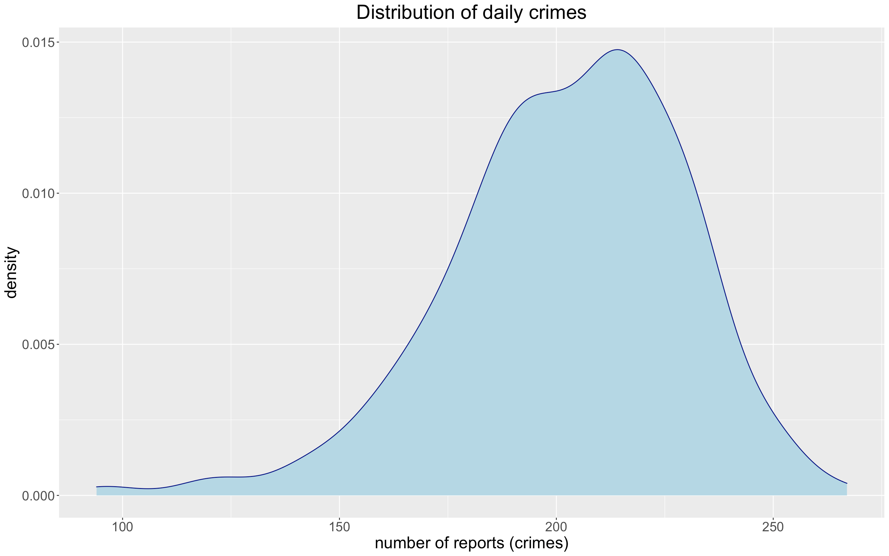 Distribution of crimes per day in Boston during 2022.
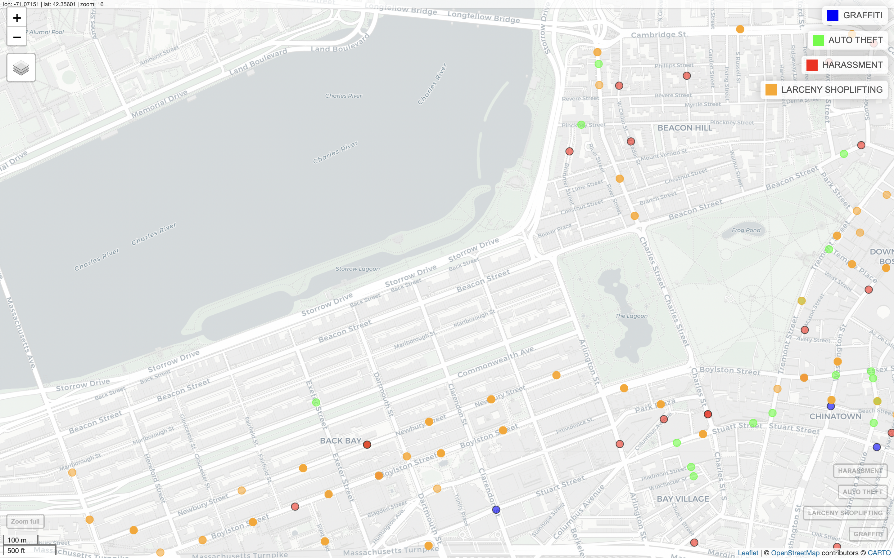 Crimes in the Back Bay area by the location in which they occured.
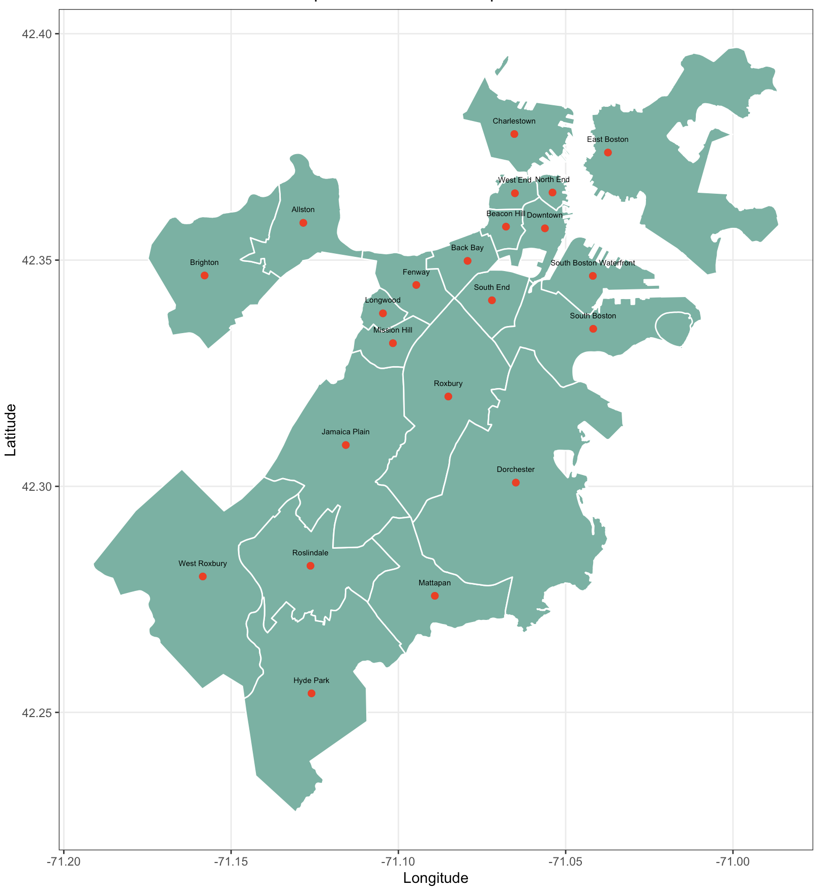 A map of Boston divided by neighborhoods.
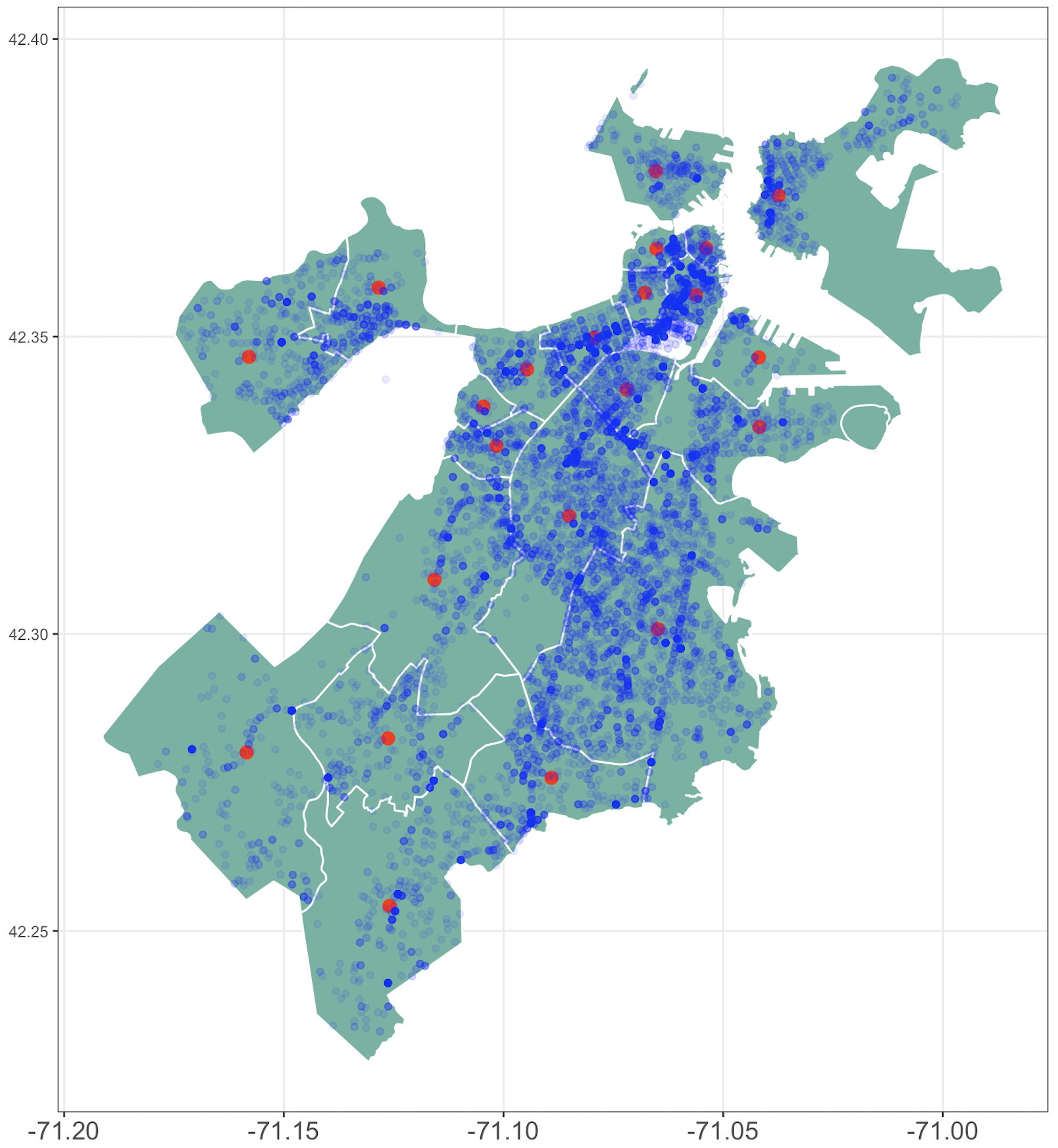 Red points are district centroids. Light blue points are locations where a crime occured.
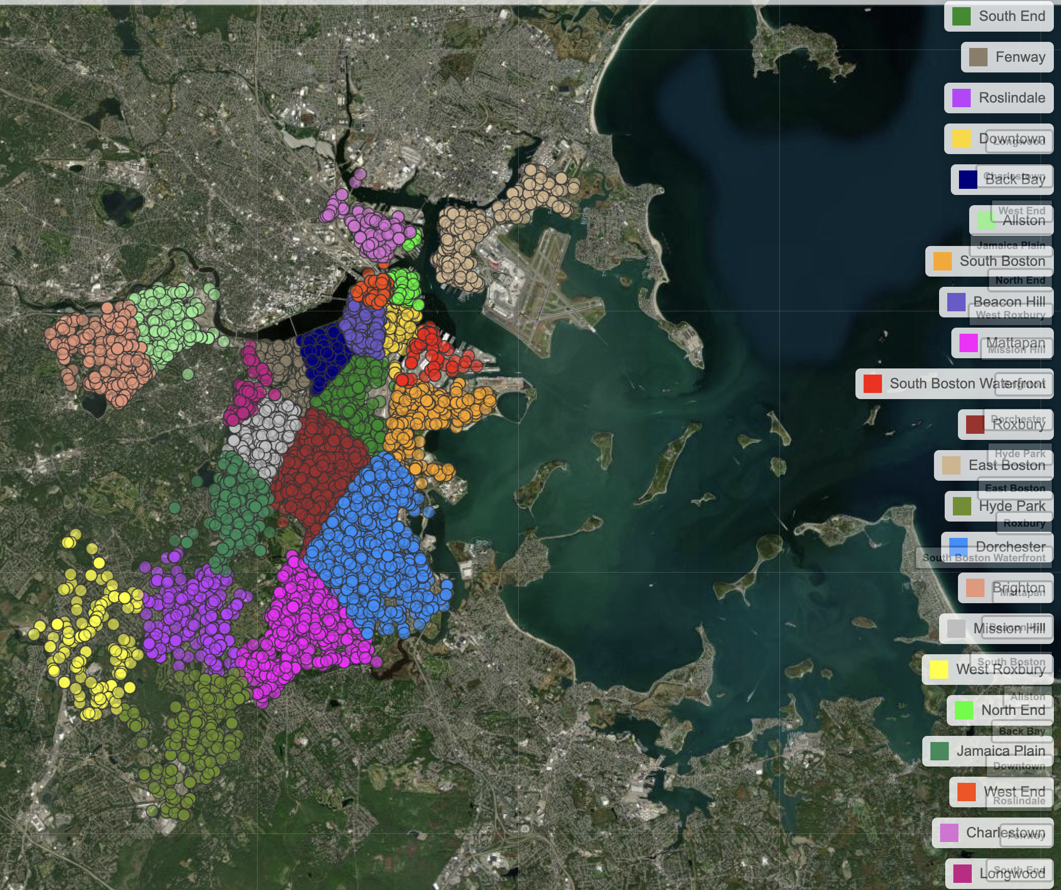 A satellite image of Boston with crime points stratified by neighborhood. The points are spread throughout almost all of the city.
Gaussian process
We are going to consider point referenced data using a Gaussian process to incorporate a spatial dependence structure within the data. If \(s_i\in \mathbb{R}^2\) denotes the coordinates of the \(i-th\) district in Boston, the regresion model that we will be using is given by:
\(\begin{equation}Y(s)=\mathbf{\mu}(s)+\mathbf{\omega}(s)+\mathbf{\epsilon}(s),\end{equation}\) with
\[\begin{equation}Y(s):=\begin{pmatrix}Y(s_1)\\Y(s_2)\\ \vdots\\ Y(s_n) \end{pmatrix},\end{equation}\] \[\begin{equation}\mathbf{\mu}(s):= \begin{pmatrix}\mu(s_1)\\ \mu(s_2)\\ \vdots\\ \mu(s_n) \end{pmatrix}, \end{equation}\]\(\mu(s_i)=\mathbf{x}(s_i)^{T}\mathbf{\beta},\) where \(\mathbf{x}(s_i)\) denotes a feature vector that contains the predictive variables for the variables associated to the i-th neighborhood and \(\begin{equation}\mathbf{\beta}=\begin{pmatrix} \beta_1 \\ \beta_2\\ \vdots \\ \beta_p \end{pmatrix}\end{equation}\)
is a vector of coefficicients.
\[\begin{equation}\mathbf{\omega}(s):=\begin{pmatrix}w(s_1)\\w(s_2)\\ \vdots\\ w(s_n) \end{pmatrix} \sim N_{n}\Big(\mathbf{0} , \Sigma(s,t)\Big)\end{equation}\]denotes a Gaussian process that corresponds to the spatial dependence structure in the data, using an exponential covariance function. That is, if \(s_i, s_j\) are the coordinates of two arbitrary districts in Boston, then
\[\begin{equation}Cov(w(s_i), w(s_j))=\Sigma(s_i,s_j)=\sigma^2exp\{ -\phi d_{i,j}\},\end{equation}\]where \(d_{i,j}:= \| s_i-s_j\|_{2}\) is the Euclidean distance between the coordinates of districts \(i\) and \(j\).
And
\[\mathbf{\epsilon}(s) :=\begin{pmatrix}\epsilon(s_1)\\ \epsilon(s_2)\\ \vdots\\ \epsilon(s_n) \end{pmatrix} \sim N_{n}\Big(\mathbf{0}, \varphi^2 I_{n\times n} \Big)\]denotes the errors which we assume to be independent of \(\mathbf{\omega}(s)\).
As a consequence of such specification, we get that
\[\begin{equation}Y(s)\sim N_{n}\Big(\mathbf{\mu}(s),\Sigma(s,t)+\varphi^2 I_{n\times n} \Big).\end{equation}\]Notice that this is a linear regresion to the mean model, given that we propose a linear combination of the feature variables which affects the mean of the response variable. We propose models of such a structure, using different explanatory variables (features), using a Bayesian approach.
Moreover, the prior distribution of the parameters \(\phi, \varphi^2, \sigma^2\) is given by a non-infomrative Gamma. It is important to keep in mind that by default, BUGS uses precision in the parametrization of the normal distribution and not the variance. For implementation purposes, we ran 2 chains of longitude \(10,000\) with a thining of 20 units and a burning period of \(1,000\) iterations with OpenBUGS.
Prediction analysis
We implemented two models: Model 1 and Model 2. Model 1 includes more variables through a dimension reduction done with PCA. Model 1 used indices as feature variables, each of which considers several variables (e.g. an education index, which considers percentage of population with a masters degree, fraction of the population who are undergrad students, etc.). Whereas Model 2 is a more parsimonious model that uses more interpretable variables.
 We used a bayesian kriging approach to make predictions. We randomly chose two districts maked in orange and kept them to make predictions unobserved during training. We used the rest of the neighborhoods to train the model.
We numbered the districts from 1 to 22, and selected two numbers randomly fixing a seed for replicaton purposes. The selected numbers (which we excluded for training and kept only for prediction purposes) were 15 and 19 corresponding to North End and South Boston Waterfront. So we predicted the values of \(Y(s_{15})\) and \(Y(s_{19})\) to test the models on these values and compare them.
We used a bayesian kriging approach to make predictions. We randomly chose two districts maked in orange and kept them to make predictions unobserved during training. We used the rest of the neighborhoods to train the model.
We numbered the districts from 1 to 22, and selected two numbers randomly fixing a seed for replicaton purposes. The selected numbers (which we excluded for training and kept only for prediction purposes) were 15 and 19 corresponding to North End and South Boston Waterfront. So we predicted the values of \(Y(s_{15})\) and \(Y(s_{19})\) to test the models on these values and compare them.
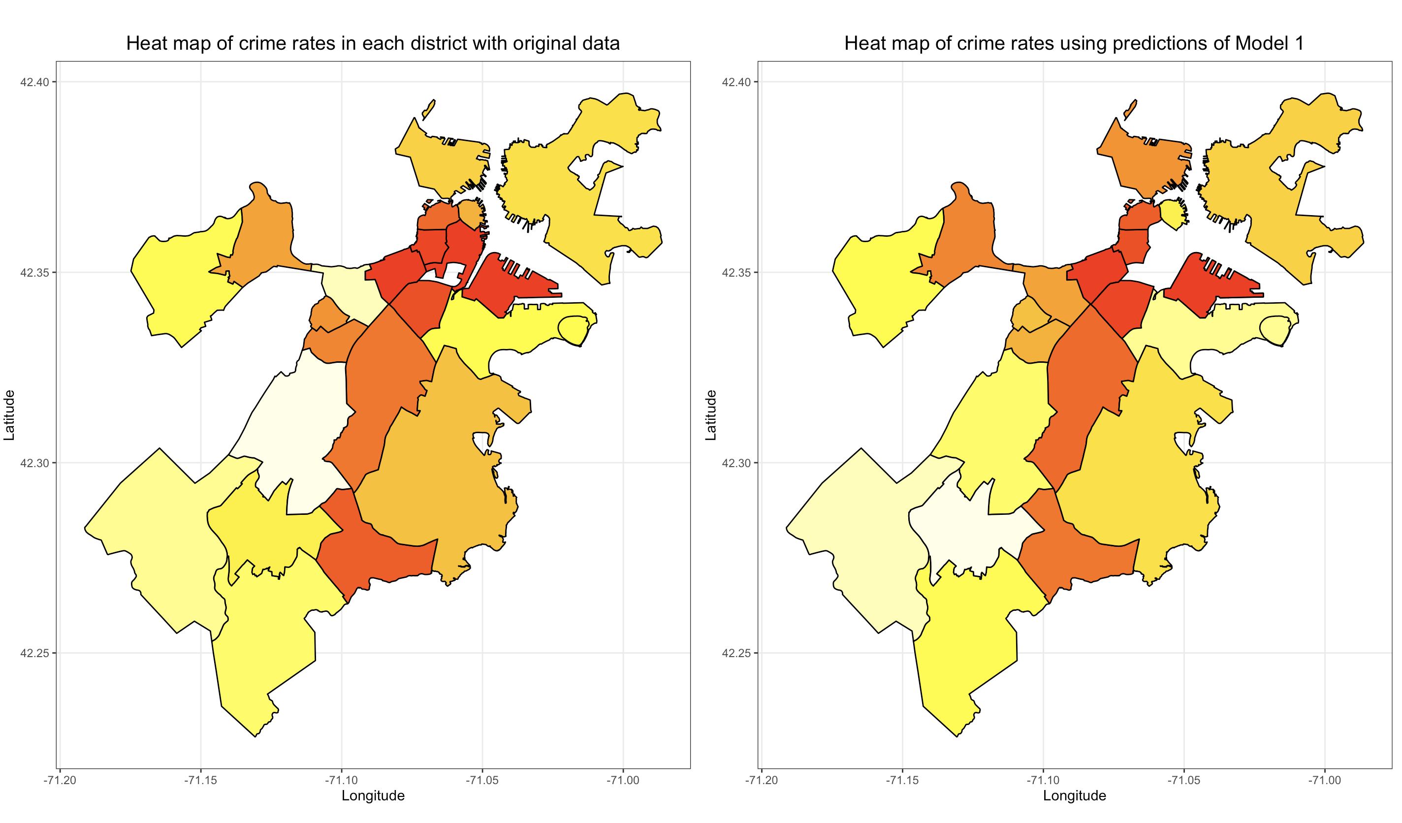 Comparison between the original crime rate heat map and the crime rate heat ma generated using the Model 1.
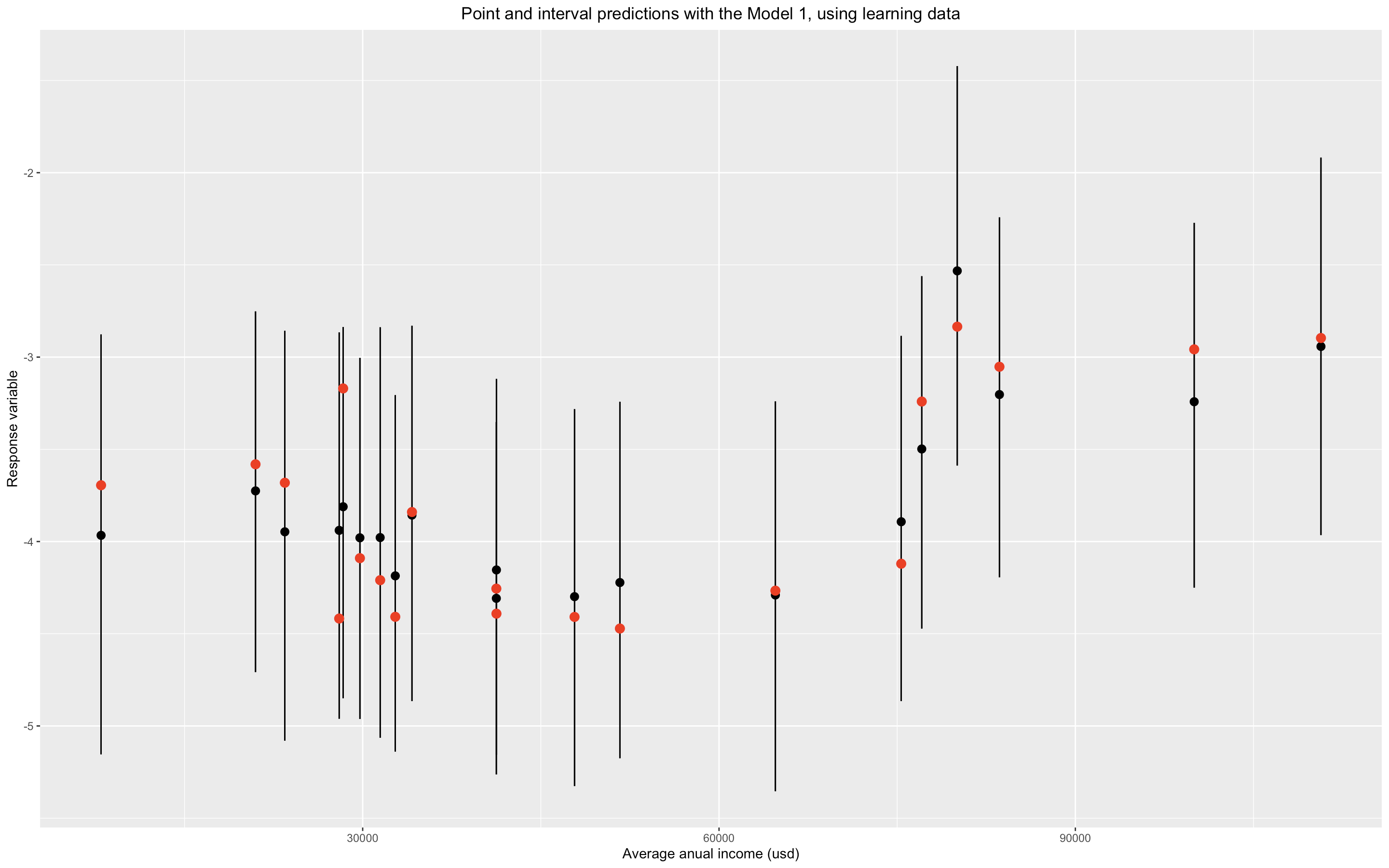 Point and prediction intervals as a function of average annual income in Boston’s neighborhoods. Red points are observed values, whereas black points are point predictions.
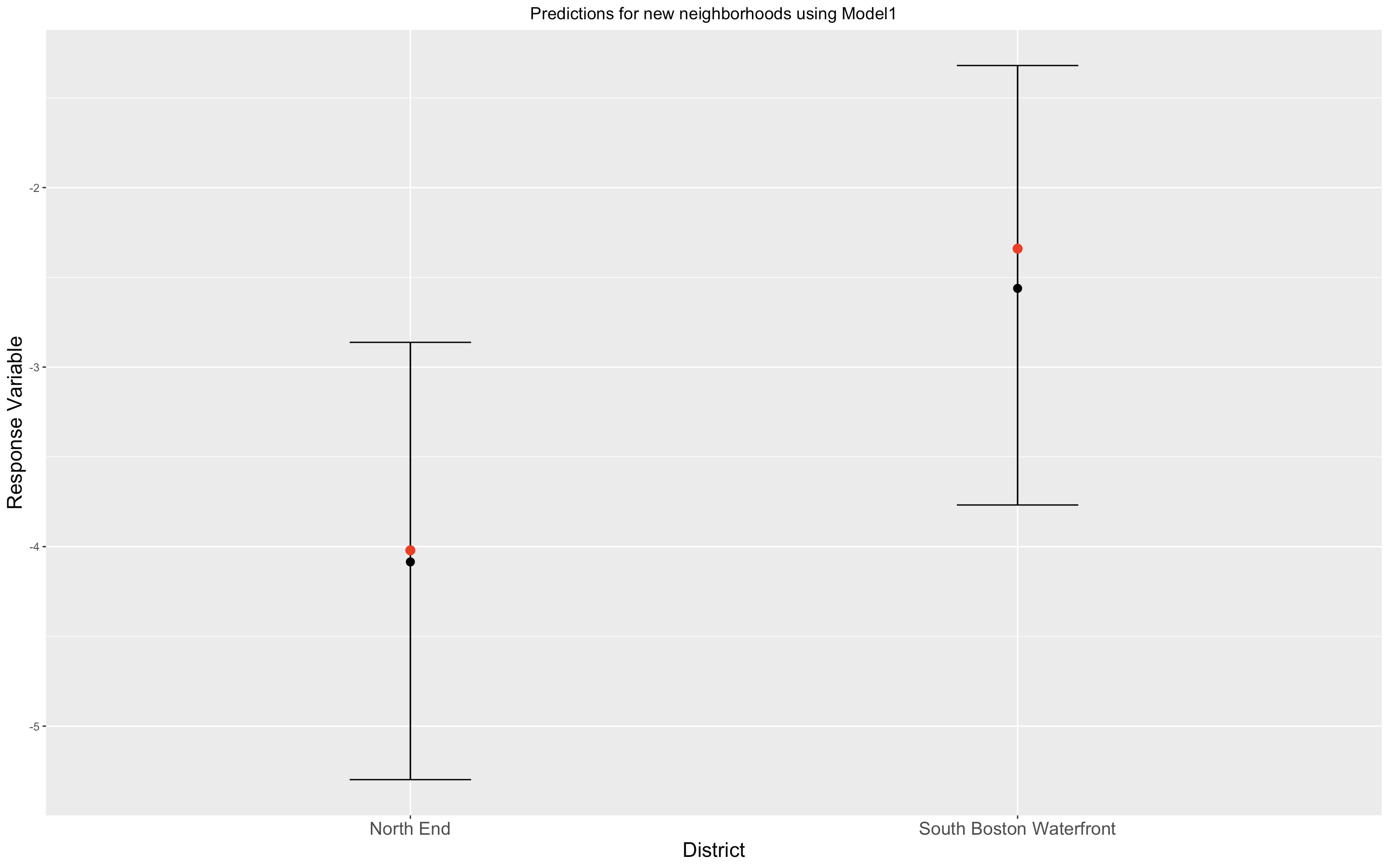 Point and interval predictions for neighborhoods that we didn’t use during training. Red points are observed values, whereas black points are point predictions.
How can we interpret these intervals in terms of crime rates? With respect to quantiles, if \(X\) is a random variable and \(q_p\) is a quantile of order \(p\) (i.e. \(q_p=inf\{t\in\mathbb{R}:\mathbb{P}(X\leq t)\geq p\}\)), then:
\[\begin{equation}0.95=\mathbb{P}(q_{0.025}\leq X\leq q_{0.975})=\mathbb{P}(e^{q_{0.025}}\leq e^X\leq e^{q_{0.975}}),\end{equation}\]since the exponential function is an increasing function , hence it doesn’t alter inequalities. We can use this result and this kind of ideas to convert every prediction (either point prediction or interval prediction) to terms of crime rates instead of crime rates in a log-scale.
We estimated such quantiles of the predictive distribution using Markov Chain Monte Carlo.
Here were report the results:
| Variable | Point prediction | \(q_{0.025}\) | \(q_{0.975}\) | Observed value | District | Model |
|---|---|---|---|---|---|---|
| \(Y(s_{15})\) | -4.09 | -5.30 | -2.86 | -4.02 | North End | Model 1 |
| \(Y(s_{19})\) | -2.56 | -3.77 | -1.32 | -2.34 | South Boston Waterfront | Model 1 |
| \(Y(s_{15})\) | -3.27 | -4.66 | -1.88 | -4.02 | North End | Model 2 |
| \(Y(s_{19})\) | -2.68 | -4.29 | -1.08 | -2.34 | South Boston Waterfront | Model 2 |
| Variable | Point prediction | \(e^{q_{0.025}}\) | \(e^{q_{0.975}}\) | Observed crime rate | District | Model |
|---|---|---|---|---|---|---|
| \(Y_{15}\) | 0.0168 | 0.0050 | 0.0572 | 0.0179 | North End | Model 1 |
| \(Y_{19}\) | 0.0772 | 0.0231 | 0.2671 | 0.0963 | South Boston Waterfront | Model 1 |
| \(Y_{15}\) | 0.0381 | 0.0095 | 0.1518 | 0.0179 | North End | Model 2 |
| \(Y_{19}\) | 0.0685 | 0.0137 | 0.3396 | 0.0963 | South Boston Waterfront | Model 2 |
Model 2
This model used a linear predictor of the form
\[\begin{equation}\mu(s_i) = \beta_{1} + \beta_{2} X_{1,i} + \beta_{3} X_{2,i} +\beta_{4} X_{3,i} + \beta_{5} X_{4,i} + \beta_{6} X_{5,i} +\beta_{7} X_{6,i} + \beta_{8} X_{7,i} + \beta_{9} X_{8,i}, \end{equation}\]where the \(X_{k,i}'\) is the \(k-\)th demographic characteristic of the district \(i\). For example,
\(X_{1,i}=\)percentageUndergrads: percentage of people in the district \(i\) that have an undergraduate degree.
\(X_{2,i}=\) percentageMasters:percentage of people in the district \(i\) that hold a masters degree.
\(X_{7,i}=\)incomePerCapita: average annual income per person in the neighborhood \(i\).
\(X_{8,i}=\)metroTren: percentage of people in the neighborhood \(i\) whose main transport is the metro or the train.
This model had a similar performance as the Model 1 with the predictions for neighborhoods that we didn’t use during training as well as with predictions with the training dataset. As it can be observed in the summary tables however, the Model 2 had smaller intervals, which makes it better in that criteria. We don’t preseent the inference for the coefficients associated to each variable, however we should emphasize tha some variables were not significant at the \(5\%\) level. For this reason we implemented a third model excluding the variables that were not significant at the \(5\%\) level, and incorporating the education index that we created with PCA. This third model had a similar performance to the Model 2, having the advantage of being more parsimonious due to the fact that it had less variables. With respect to the variables that had a considerable predictive capactity (significant at the \(5\%\) level) with Model 2, we obtained the annual income oper capita has a strong significance.